Approximating Non-linear Functions

Imagine a tool so versatile that it can learn to recognize patterns, make decisions, and even mimic human-like reasoning. This tool isn’t a product of science fiction, but a reality in the world of computer science known as a neural network. At its core, a neural network is inspired by the intricate web of neurons in our brains, but instead of processing thoughts and memories, it processes data and learns patterns.

As universal function approximators, neural networks combine linear transformations with non-linear activation functions, gaining the ability to approximate any continuous function. This powerful combination allows them to model intricate patterns and relationships in data, making them a cornerstone of deep learning.

But why is this capability so significant? In the vast realm of data-driven tasks, from voice recognition to predicting weather patterns, the underlying relationships are often complex and non-linear. Traditional linear models fall short in capturing these intricacies. Neural networks, with their layered architecture and non-linear activation functions, rise to the challenge, offering a flexible and powerful approach to model these relationships.

Let’s use a simple example to illustrate the power of combining linear and non-linear layers.

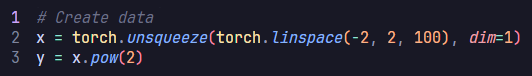
Suppose we want to approximate the function $f(x)=x^2$ using a neural network. This is a simple non-linear function. If we use only linear layers, our network won’t be able to approximate this function well. But by introducing non-linearity, we can achieve a good approximation.

1. Using Only Linear Layers

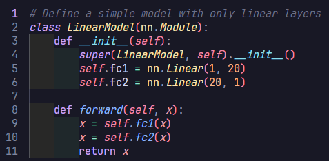
Let’s first try to approximate $f(x)=x^2$ using only linear layers.

Creating data:

Defining the linear neural network:

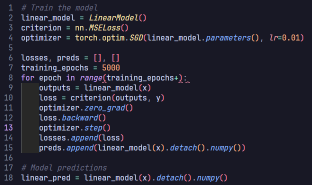
Training the neural network:

Visualizing the learning process:

We observe that the linear model doesn’t approximate the function $f(x)=x^2$ well, even after 5000 epochs. This is because linear transformations are great for scaling, rotating, and translating data. However, no matter how many linear layers we stack together, the final transformation will always be linear. This means that the expressive power of the network remains limited.

2. Introducing Non-linearity

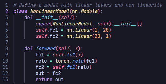
Now, let’s introduce a non-linear activation function (ReLU) between the linear layers. These non-linearities allow the network to model complex, non-linear relationships in the data.

Defining the Non-linear network:

Training the neural network:

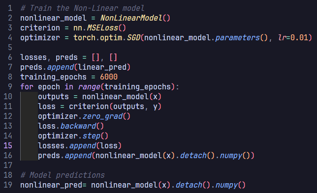
Visualizing the learning process:

With the introduction of non-linearity, the network can now approximate the function $f(x)=x^2$ much better.

3. Combining Linear and Non-linear Layers

When we combine linear layers with non-linear activation functions, the magic happens:

• Expressive Power: By interleaving multiple linear layers with non-linear activations, the network gains the capability to approximate complex functions. Each successive layer refines and builds upon the features extracted by its predecessor layer.

• Hierarchical Feature Learning: Deep networks learn hierarchical features. Initial layers tend to learn simple patterns (such as edges in images), whereas deeper layers synthesize these simple features into more complex representations (like entire objects or shapes).

• Universal Approximation Theorem: This theorem states that a feed-forward network with just a single hidden layer containing a finite number of neurons can approximate any continuous function on compact subsets of $\mathbb{R}^n$, under mild assumptions on the activation function. The depth and width of the network determine its capacity to approximate complex functions.

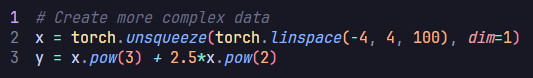
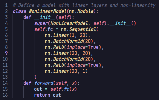
To elucidate this, let’s consider an even more complex non-linear function $f(x)=x^3+2.5x^2$. Let’s also create a deeper feedforward neural network and observe how it can approximate the non-linear function. The network architecture consists of a sequence of linear layers interspersed with batch normalization and activation functions. Here’s a step-by-step break down:

Creating data:

Defining the deep neural network:

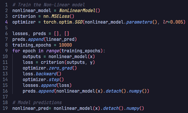
Training the deep neural network:

Visualizing the learning process:

The function $f(x)=x^3+2.5x^2$ has curves and non-linear relationships. The combination of linear layers and activation functions in the neural network allows it to “learn” these curves. By adjusting its weights through training, the network finds the best way to “bend” and “shape” its transformations to get as close as possible to this function across the input domain you’re interested in.

Intuition

Imagine trying to fit data points with just straight lines (linear functions). You’d be quite limited. Now, introduce curves (non-linearities) to your toolkit. Suddenly, you can fit a much wider variety of shapes and patterns. In essence, the combination of linear transformations and non-linear activations gives neural networks the flexibility to “bend” and “shape” their output to approximate any given function.

Takeaways

The combination of linear and non-linear layers allows the neural network to form complex decision boundaries and represent non-linear relationships. In our examples, the non-linear model can bend and adjust its shape to fit the curve of the non-linear functions $f(x)=x^2$ and $f(x)=x^3+2.5x^2$, while the purely linear model can only produce straight lines and cannot fit the curve.

While the examples provided might seem basic, they serve a crucial purpose. Truly grasping the concept that neural networks can approximate any continuous function offers a deeper and more profound understanding of why deep learning models are so versatile and powerful.

I hope these visualizations help shed light on the underlying principles of neural networks. They were certainly helpful to me.